

Methodologies for the evaluation of spatial representativeness of air quality monitoring stations in Italy
ENEA is supporting the Italian Ministry of Environment, Territory and Sea in building the National Network of Special Purpose Monitoring Stations. In this framework, ENEA is carrying out an assessment of the spatial representativeness of the selected monitoring sites, to be used in model validation, data assimilation tools and population exposure studies.
Given that a standard procedure is not yet recognised at the international level, in this study different methodologies are being applied in the Italian territory in order to find out one or more fit-to-purpose approaches to spatial representativeness. Three methods are explored based on: 1) statistical assessment of objective factors (land cover, population distribution, orography, etc.); 2) assessment of variability of emissions; 3) assessment of 4D Eulerian concentration field and gradients from model simulations. Specific datasets produced by the Italian Integrated Assessment Modelling System (MINNI) are being used for this purpose.The three methods cover different assessment situations and targets: primary and secondary pollutants, availability of model datasets or measured concentration time series, urban and rural stations. The preliminary results of their application to selected pollutants and monitoring sites are here presented and discussed. The principal strengths and weaknesses of each method are reported in relation to the assessment of the spatial representativeness of existing monitoring sites or to the planning of new monitoring networks
Metodologie per la valutazione della rappresentatività spaziale di stazioni di monitoraggio della qualità dell’aria in Italia
La rappresentatività spaziale e temporale dei siti di monitoraggio delle concentrazioni di inquinanti in atmosfera è un parametro fondamentale nella scelta della dislocazione delle stazioni di misura e nelle valutazioni di esposizione della popolazione ai livelli di concentrazione misurati.
Poiché non esiste in letteratura una metodologia consolidata al riguardo e riconosciuta a livello internazionale, in questo studio è descritta l’applicazione di tre originali approcci metodologici per la valutazione della rappresentatività spaziale di siti di monitoraggio della qualità dell’aria. I dati utilizzati per la valutazione provengono dai prodotti del Sistema Modellistico Nazionale MINNI disponibili a scala chilometrica su tutto il territorio Italiano. In questo lavoro vengono presentati i risultati preliminari dell’applicazione di tali metodi a specifici inquinanti e siti sul territorio, discutendone criticamente le principali potenzialità e i limiti. Gli inquinanti considerati sono sia primari che secondari e la tipologia delle stazioni di misura analizzate sono quelle di fondo urbano e rurale
Gaia Righini, Andrea Cappelletti, Irene Cionni, Alessandra Ciucci, Giuseppe Cremona, Antonio Piersanti, Lina Vitali, Luisella Ciancarella
In order to describe the complex spatial and temporal patterns of atmospheric pollution in a specific area and to achieve a cost-effective control of air quality, the spatial and temporal representativeness of an air quality monitoring station is of fundamental importance.
According to literature, the spatial representativeness of a monitoring site is related to the variability of concentrations of a specific pollutant around the site. For example in Larssen et al. (1999) the area of representativeness is defined as “the area in which the concentration does not differ from the concentration measured at the station by more than a specified amount”. In Spangl et al. (2007) the definition of representativeness is based on the comparison of concentration values observed at two different sites: “A monitoring station is representative of a location if the characteristic of the differences between concentrations over a specified time period at the station and at the location is less than a certain threshold value.” A similar definition, frequently mentioned in the literature and particularly useful to compare observed data with model simulations, is the one adopted by Nappo et al. (1982), obtained comparing point measurements with observations in a large area (or volume). As the concentration of each pollutant depends on several factors (namely, the variation of meteorological conditions, local sources, topography, transport and chemical reactions) the spatial representativeness is expected to vary not only on a temporal basis (annual, seasonal and daily variability) but also for each pollutant of interest.
The assessment of station spatial representativeness can be based on various sources of information but a standard procedure that can be applied to different monitoring networks in different regions is not recognised at the international level. In this framework, the European working groups AQUILA (Air Quality Reference Laboratories) and FAIRMODE (Forum for Air Quality Modelling in Europe), technically supporting the implementation of 2008/50/EC Directive on ambient air quality and cleaner air for Europe (Air Quality Directive), are promoting the discussion concerning spatial representativeness of monitoring data starting from the most popular methods used in literature. Recently, FAIRMODE addressed a specific recommendation to the European Commission concerning the review of the EU Air quality policy, encouraging further competence building on this topic (http://fairmode.ew.eea.europa.eu/guidance-use-models-wg1/directive-revision/fairmode-recomm_final.docx).
Therefore, the assessment of spatial representativeness of air quality monitoring stations is a prevailing issue of prominent scientific interest at the national and international levels.
On the national level, in the framework of the Italian Legislative Decree 155/2010 for the compliance with the Air Quality Directive, a Cooperation Agreement for starting up the Italian National Network of Special Purpose Monitoring Stations was signed in 2011 by the Italian Ministry for the Environment, the Territory and the Sea (MATTM), the Italian National Agency for New Technologies, Energy and Sustainable Economic Development (ENEA), the National Research Council (CNR) and the Italian Istituto Superiore di Sanità (ISS). In the frame of this agreement, one of ENEA’s tasks is to assess the spatial representativeness and geographical area of concern for each selected monitoring station. Figure 1 shows, for all pollutant, the position of the selected measuring stations.
According to the state of the art assessment of spatial representativeness, four different methodological approaches are examined by ENEA for detailed analysis: a statistical method based on objective factors, a method based on the knowledge of the spatial distribution of emissions, a method based on model simulated concentration fields, and finally a method based on the analysis of backward trajectories.
In this work, the preliminary results of the first three methods applied to selected pollutants and monitoring sites are presented, and the principal strengths and drawbacks are discussed. Each of the three methods has been the object of a detailed technical report (Cremona et al., 2013; Piersanti et al., 2013; Vitali et al., 2013). Presently studies are in progress for a fourth method, to be completed by June 2013; therefore, a final assessment of the most suitable methods for the Italian monitoring network will be carried out in the last stage of the project.
All methods except the first were implemented by using specific datasets produced by MINNI (www.minni.org), which is the Italian Integrated Assessment Modelling System (AMS) for supporting the International Negotiation Process on Air Pollution and assessing Air Quality Policies at the national/regional level (Mircea et al. 2011). The AMS simulates 3-dimensional meteorology and air quality fields for the entire Italian territory, on a national domain (20 km resolution on horizontal grid) and on 5 nested regional domains (4 km resolution on horizontal grid). Yearly simulations are available for several years: 1999, 2003, 2005, 2007. The model implements an integrated and multi-pollutant approach for calculating hourly concentrations of all pollutants regulated by the Air Quality Directive (SO2, NO2, ozone, PM10, PM2.5, NH3, Heavy Metals, PAHs, etc.) plus the depositions of sulphates and nitrates.
Method 1: objective factors (Land Cover)
A first methodological approach relies on a simplified description of atmospheric pollution processes: an empirical relationship is assumed between physical objective factors influencing air pollution (i.e., wind direction and speed, orography, land cover, urbanized areas, large point emission sources) and concentrations recorded by air quality monitoring stations. This approach is widely used in air quality assessment, particularly when insufficient data on emissions and meteorology, and/or limited resources are not adequate for a detailed representation of pollution processes.
In our study, we chose to analyze land cover near monitoring stations, relying on a causal relationship with concentrations: land cover patterns are representative of actual locations of emissions (i.e., urban areas concentrate heating and traffic emissions, forests are responsible of biogenic VOCs, agricultural areas are the sites of waste biomass burning and NH3 vaporization from manure fertilizers), and emissions are the main cause of concentrations. Using land cover to assign a georeferenced location to aggregated values recorded in emission inventories is a common practice in air quality modelling.
In compliance with literature studies, in particular Janssen et al. (2012), we developed a synthetic, pollutant-dependent, indicator β for the dependency of concentration on land cover, and we studied how β is varying in the neighbourhood of the selected monitoring site. The formulation is
![]()
where, assuming a reference area around the monitoring site, CLi is the fraction of the area corresponding to CLi class of land cover and i is a weight coefficient, determining the influence of CLi class as a potential determinant of pollutant concentration. The factor β is therefore an indicator of “land cover polluting power”. The rationale is that, the more variable is β in the surroundings of the site, the less representative of the air quality in the surroundings of the site are the concentrations measured at the station.
For determining CLi values, we used Corine Land Cover 2006 database (ISPRA, 2010a), with ad-hoc improvements by means of an aggregation of the original 44 classes into 11 CLi classes and an integration of the road network class, using more detailed layers with national coverage. Spatial treatment of land cover was performed with the help of GIS (Geographical Information Systems) software.
The i coefficients are calculated from a statistical optimization of the function C(β)=nβ2+mβ+q, where the dependency of the concentration C on the land cover indicator β is explicated. The optimization was carried out by a multivariable regression on measured concentration values from the national database of air quality measurements (ISPRA, 2010b), using 2007 annual averages. Since the optimization relies on measured concentrations, ai are pollutant-dependent. The computing was performed by the statistical code R (http://www.r-project.org/).
After the calibration, the calculation of β was performed for 10 monitoring stations for PM2.5 and 12 monitoring stations for ozone or precursors, using a circular buffer with 2 km radius centred at each station as the area of influence for the measuring site. At this point, the calculation of β was performed for increasing radii (5, 7.5, 10 km), as shown in Figure 2, obtaining an array of values for each station. Finally, spatial representativeness of the station has been quantitatively assessed comparing each buffer’s β value with the “station” value (in the 2 km radius buffer): a difference of less or more than 20% indicates whether or not the station measurement represents the concentration value inside the buffer.
In this analysis a threshold value of 20% was set according to literature (Blanchard et al. 1999; Janssen et al. 2008a) and since it is compatible with the quality objectives for most monitoring data included in the Air Quality Directive (15% and 25%, depending on the measured pollutant).
Generally, this approach is useful when annual time series of measured concentrations are available from a consolidated and spatially uniform monitoring network, allowing a good calibration of β. Moreover, using a high-resolution land cover database allows detailed assessment of spatial representativeness, very useful for urban and suburban monitoring sites, where land cover is highly variable. On the other hand, the robustness of the results is strongly dependent on the quality of the calibration dataset (spatial coverage, consistency and coverage of recordings), and the assessment is limited to annual concentrations, due to the absence of meteorological input capable of following daily and seasonal variations.
Method 2: emissions variability
The second method is based on the correlation between the spatial distribution of atmospheric concentrations of pollutants and the corresponding emission distribution. This is a simplified modelling approach, using a linear relationship between emissions and concentrations. On the other hand, simplifications lead to a fast and reliable assessment of representativeness, using emission inventory data, more commonly available at wide spatial coverage than concentration data. The principle is to define an inversely proportional relation between emission variability around a monitoring site and its spatial representativeness: high emission variability means low spatial representativeness, whereas low emission variability means high spatial representativeness.
A similar approach is reported in Henne et al. (2010), where surface fluxes of pollutants are studied to determine representativeness areas of monitoring sites using a proxy variable (population) in place of the emissions. In our work we actually used emissions data, taking advantage of the MINNI atmospheric modeling system. Here, a gridded emission inventory at national scale is provided, with disaggregation (in space, time, chemical speciation and aerosol size profile) for mesoscale Chemical Transport Modeling.
The analysis of emission spatial variability was performed by GIS, applying a “neighbourhood statistics” algorithm: for each grid point, the amount of variation in emission values among neighbour cells was derived (range function). Therefore, each point of the calculation grid was given a unique value synthesizing how significantly the emissions vary around the grid point.
As MINNI dataset covers a wide range of reference situations, the methodology was applied on 2 different emission inventory sources: the national emission inventory (ISPRA, 2009), annually compiled for fulfilment of UNECE CLRTAP international agreements, and the national GAINS emission estimates (D’Elia et al., 2009), deriving from GAINS Europe scenario analysis methodology. In both cases, 2005 is the reference year. Moreover, different time intervals for emission integration were tested (whole year, summer, winter). The analyses were performed on primary pollutants since this simplified modelling approach excludes secondarily generated fractions.
As a result, more than 80 output maps were generated and evaluated in GIS environment, where they have been integrated with thematic layers, useful for understanding the reasons of emission variations near the selected station. Each map is referred to a MINNI modeling domain, covering Italian macroregions: as an example, Figure 3 shows PM2.5 emission variability in the North-East of Italy.
Figure 4, at a higher spatial detail, shows PAHs emission variability for Ripatransone station. Light areas (reporting low variability values) prevail around the station, and dark areas (high variability values) are located far from the station and over cities (Ascoli Piceno 21 km SW, Teramo 35 km S). Then, the more detailed evaluation is semi-quantitative and based on an automatic classification of range of values (natural breaks): the two lowest ranges (corresponding to high representativeness) cover the station grid cell and a large area around (about 103 km2), extended in all directions but excluding cities, where emission variability is in the highest ranges. This means that, for this station, spatial representativeness is high but does not include cities.
Method 3: concentration similarity
The third selected approach to the evalation of representativeness is the most straightforward: the concentrations recorded at the site of interest are directly compared with concentrations recorded at selected points in the surrounding area, in a fixed time interval. The monitoring station is representative of a wider area if all measurements in this area differ by less than a threshold from the station measurements.
For a quantitative assessment of spatial representativeness of atmospheric monitoring stations, Nappo et al. (1982) give a useful and detailed definition: “a point measurement is representative of the average in a larger area (or volume) if the probability that the squared difference between point and area (volume) measurement is smaller than a certain threshold more than 90% of the time”.
The availability of field measurement campaigns, covering a main site and different points around it, is very limited, due to costs and complexity of instrumental setups. On the contrary, air quality models, running on large spatial domains and for long time ranges, routinely produce 4D concentration fields (3 spatial dimensions and time), useful for comparing concentration values at a selected site and in the surroundings. Therefore, as done for method 2, we applied the methodology by adopting the MINNI model dataset, providing concentration fields for all pollutants regulated by law.
On the methodological basis proposed by Nappo et al. (1982), assuming the model concentrations as “measurements”, we developed a procedure for recursively comparing the annual concentration time series. At each time step, the difference between the concentration values measured at the site of interest (coordinates Xsite,Ysite,Z0) and at each grid point (coordinates x,y,Z0) in the model domain has been calculated. A threshold value of 20% was set, following the choice explained in Method 1 paragraph, for the difference between concentrations, in order to assess the condition of “concentration similarity”.
A 2-dimensional frequency function fsite(x,y), specific of each site of interest, counting positive occurrences of “concentration similarity” for each grid point of the model domain, was defined and finally spatial representativeness area of the site of interest was assessed (i.e. fsite(x,y)>0.9 is verified).
With the help of Unix and NCL (Zender, 2008) scripting, the frequency function fsite(x,y) was calculated, stored (in NetCDF files) and mapped (in image files). Results data were finally imported in GIS software and overlayed with thematic layers, useful for studying concentrations variation around the selected station.
The described procedure was applied on model results for PM10, PM2.5 and ozone, all having a relevant secondary component.
As MINNI model dataset covers a wide range of reference situations, a detailed sensitivity analysis was performed on input data: different meteorological years and emission inventory sources, producing different concentration fields, were used for assessing representativeness at the selected stations. Furthermore, the variation of fsite(x,y) corresponding to variations in the time averaging of concentrations was tested, in compliance with the Air Quality Directive requirements for each pollutant. Seasonal representativeness assessment variability was also evaluated. Overall, more than 500 statistical products were generated by the recursive application of the procedure.
An example of the obtained results is shown in Figure 5, concerning ozone measurement representativeness assessment at San Pietro Capofiume station (Eastern Po Valley, Northern Italy). Figure 5 shows fsite(x,y) values integrated with supporting thematic layers. Representativeness area (fsite(x,y)>0.9) is immediately visible in pink colour tones and can be precisely determined (x model grid cells, i.e. y km2).
Comprehensively, the method shows very good performances in describing both the extension and the shape of representativeness areas, with spatial resolution of results (i.e. fsite(x,y) functions) being the same as the input data used for the assessment.
Conclusions
In the framework of the implementation of the Italian Special Purpose Monitoring Network for air quality, ENEA has been testing different methodologies for the evaluation of spatial representativeness of monitoring stations, in order to study how point measures at a single site reflect pollutant concentrations in the area surrounding the site. At present, 3 methodologies were tested, covering different typologies of input datasets and assessment algorithms.
Method 1, based on using land cover data as a proxy variable of concentration, allows to determine spatial variations of the polluting factor in analysis, at increasing distance from the selected site. The empirical relationship has a simplified formulation, therefore the quality of results strongly depends on the selected dataset of measured concentrations, used in the calibration stage. The method looks promising for evaluating urban monitoring sites, due to the availability of free high resolution datasets of land cover, describing accurately urban environments.
Method 2, using MINNI gridded emission database to analyze emission variability as a proxy variable of concentration, gives a complete picture of spatial variations of the polluting factor in analysis, covering the whole model domain, thus not depending on any monitoring site. This is useful for a comprehensive evaluation of spatial representativeness, e.g. for designing new monitoring networks, though some limits are present (just primary pollutants, semi-quantitative evaluation).
Method 3, directly comparing hourly concentrations at the selected site and in the surrounding by using MINNI gridded concentration database, shows encouraging skills in accurate definition of representativeness area and shape. The method proved to be particularly robust, as the comparison is performed at high time resolution and no proxy variable is used. As for method 2, using a gridded model means that representativeness is evaluated at the spatial detail of the model grid, not allowing for example an adequate description of urban stations.
The three methods were designed to cover different assessment situations and targets: primary (methods 1 and 2) and secondary (method 3) pollutants, availability of model datasets (method 2 and 3) or measured concentrations time series (method 1), urban (method 1) and rural (method 2 and 3) stations. At present, a fourth method, based on backward trajectories of air masses reaching the selected site, is under development, relying on meteorology as a proxy variable of air pollution. In a following phase, the four methods will be applied to all stations of the Special Purpose Monitoring Network, to derive a final evaluation of spatial representativeness.
This research covers a very topical issue at the national and international levels, with a great effort aiming to test strengths and weaknesses of several state-of-the art assessment methodologies. Some specific developments, mostly targeting flexibility in input datasets usage, have been realized and others are ongoing, thus giving promising and innovative materials for a better knowledge of air quality monitoring potential and limits.
Acknowledgments
This work is part of the Cooperation Agreement for starting up the Italian National Network of Special Purpose Monitoring Station, funded by the Italian Ministry for Environment and Territory and Sea, which the authors wish to thank also for providing MINNI project results.
The authors wish to thank Felicita Russo (ENEA) for reviewing this paper.
References
Blanchard C.L., Carr E.L., Collins J.F., Smith T.B., Lehrman D.E., Michaels H.M., (1999), “Spatial representativeness and scales of transport during the 1995 integrated monitoring study in California’s San Joaquin Valley”, Atmospheric Environment, 33, 4775-4786.
Cremona G., Ciancarella L., Cappelletti A., Ciucci A., Piersanti A., Righini G., Vitali L. (2013), “Rappresentatività spaziale di misure di qualità dell’aria. Valutazione di un metodo di stima basato sull’uso di dati emissivi spazializzati”, ENEA Technical Report, RT/2013/2/ENEA.
D’Elia I., Bencardino M., Ciancarella L., Contaldi M., Vialetto G. (2009), “Technical and Non Technical Measures for Air Pollution Emission Reduction: the Integrated Assessment of the Regional Air Quality Management Plans through the Italian National Model”, Atmospheric Environment, 43, 6182-6189.
Henne S., Brunner D., Folini D., Solberg S., Klausen J., Buchmann B. (2010), “Assessment of parameters describing representativeness of air quality in-situ measurement sites”, Atmospheric Chemistry and Physics, 10, 3561-3581.
ISPRA (2009), “La disaggregazione a livello provinciale dell’inventario nazionale delle emissioni. Anni 1990-1995-2000-2005”, Rapporto ISPRA, 92/2009, ISPRA, Roma.
ISPRA (2010a), “Uso e copertura del suolo: il progetto CORINE LAND COVER”, http://www.sinanet.isprambiente.it/it/coperturasuolo
ISPRA (2010b), “Annuario dei dati ambientali 2010”, ISPRA, Roma.
Janssen S., Deutsch F., Dumont G., Fierens F., Mensink C. (2008a), “A Statistical Approach for the Spatial Representativeness of Air Quality Monitoring Stations and the Relevance for Model Validation”, Air Pollution Modeling and Its Application XIX, 452-460, C. Borrego and A.I. Miranda (eds.), Springer Science.
Janssen S., Dumont G., Fierens F., Deutsch F., Maiheu B., Celis D., Trimpeneers E. and Mensink C. (2012), “Land use to charachterize spatial representativeness of air quality monitoring stations and its relevance for model validation”, Atmospheric Environment, 59, 492-500.
Larssen S., Sluyter R. and Helmis C. (1999), “Criteria for EUROAIRNET – The EEA Air Quality Monitoring and Information Network”, Technical report EEA, 12/1999, European Environment Agency.
Mircea M., Briganti G., Cappelletti A., Vitali L., Pace G., D'Isidoro M., Righini G., Piersanti A., Cremona G., Cionni I., Silibello C., Finardi S., Calori G., Ciancarella L. and Zanini G. (2011), “Ozone simulations with atmospheric modelling system of MINNI project: a multi year evaluation over Italy”, Proceedings of the 14th International Conference on Harmonisation within Atmospheric Dispersion Modelling for Regulatory Purposes (HARMO 14), 52-56, J.C. Bartzis, A. Syrakos, S. Andronopoulos (eds.).
Nappo C. J., Caneill J. Y., Furman R. W., Gifford F. A., Kaimal J. C., Kramer M. L., Lockhart T. J., Pendergast M. M., Pielke R. A., Randerson D. , Shreffler J. H. and Wyngaard J. C. (1982), “The Workshop on the Representativeness of Meteorological-Observations, June 1981, Boulder, Colorado”, Bullettin of the American Meteorological Society, 63, 761–764.
Piersanti A., Ciancarella L., Cremona G., Righini G., Vitali L. (2013), “Rappresentatività spaziale di misure di qualità dell’aria. Valutazione di un metodo di stima basato su fattori oggettivi”, Technical Report ENEA, RT/2013/1/ENEA.
Spangl W., Schneider J., Moosmann L. and Nagl C. (2007), “Representativeness and classification of air quality monitoring stations – Final Report”, Umweltbundesamt report, Umweltbundesamt, Vienna.
Vitali L., Ciancarella L., Cionni I., Cremona G., Piersanti A., Righini G. (2013), “Rappresentatività spaziale di misure di qualità dell’aria. Valutazione di un metodo di stima basato sull’analisi dei campi di concentrazione simulati dal modello nazionale MINNI”, Technical Report ENEA, RT/2013/3/ENEA.
Zender C.S (2008), “Analysis of self-describing gridded geoscience data with netCDF Operators (NCO)”, Environmental Modelling & Software, 23 (10–11), 1338–1342.
Gaia Righini, Andrea Cappelletti, Irene Cionni, Alessandra Ciucci, Giuseppe Cremona, Antonio Piersanti, Lina Vitali, Luisella Ciancarella - ENEA, Technical Unit Models, Methods and Technologies for Environmental Assessments
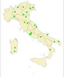
FIGURE 1 - Italian National Network of Special Purpose Monitoring Stations
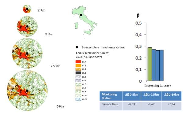
FIGURE 2 - Example of land cover buffering around Firenze-Bassi station, with calculation of β and evaluation of β variability with increasing radiuses
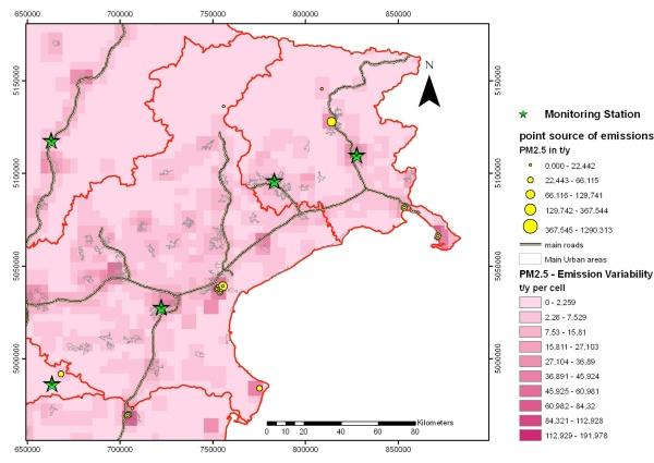
FIGURE 3 - PM2.5 emission variability (pink cells) in the North-East of Italy
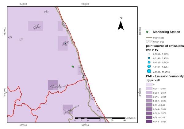
FIGURE 4 - PAHs emission variability (violet cells) around Ripatransone background rural station (green star in the center). Approximate area of representativeness is in the two lightest colour ranges
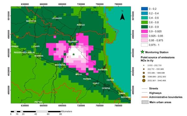
FIGURE 5 - Frequency function fsite(x,y) for San Pietro Capofiume station. Representativeness area is in pink and white